Maximum flow and the escape problem

Last weekend, my journey across the world of graphs reached its conclusion as I completed the “Maximum Flow” chapter of Introducton to Algorithms. After this, I think I will set algorithms aside for the rest of the year and let all that newly acquired knowledge sink in (or more likely just forget everything but I prefer to look at it optimistically).

When it comes to solving the maximum flow problem, the go-to algorithm is usually Ford-Fulkerson. Writing (or even just reading) a fully-fleshed Ford-Fulkerson implementation can be a painstaking task as it’s easy to get lost in the details. But the general idea behind it is reasonably easy to grasp. Ford-Fulkerson uses a greedy approach: as long as we find a path from the source vertex to the sink vertex with some available capacity, we use that capacity and send flow through it. This leaves a “residual graph” with “residual capacity” that we can use to “augment” the path further. We keep iterating until there is no path anymore in the residual graph. Here is a very nice introduction to get familiar with the specifics.

What is remarkable with maximum flow algorithms is that they can be applied to a very broad range of problems, including problems that might seem unrelated at first sight. Like the following one.

The escape problem

Problem Statement

An n x n grid is an undirected graph consisting of n rows and n columns of vertices as shown in the figures below. We denote the vertex in the ith row and the jth column by (i, j). All vertices in a grid have exactly four neighbours, except for the boundary vertices, which are the points (i, j) for which i = 1, i = n, j = 1 or j = n.

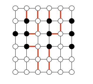
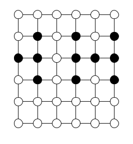
Given m <= n² starting points (x₁, y₁), (x₂, y₂),…,(x_m, y_n) in the grid, the escape problem is to determine whether or not there are m vertex-disjoint paths from the starting points to any m different points on the boundary. For example the first grid below has an escape (shown in red), but the second one does not.

escape-1 escape-2

Describe an efficient algorithm to solve the escape problem, and analyse its running time.

Solution

I will start this section with a disclaimer: I slightly changed the problem statement in order to make my life easier.

The problem states that the paths must be vertex-disjoint. In order to modelise this problem as a maximum flow problem, we would have to consider that vertices have a unit capacity. However the Ford-Fulkerson algorithm applies on maximum flow problems modelised with edge capacity. There is a small trick one can do to transform a maximum flow problem with vertex capacity to a maximum flow problem with edge capacity, which you can read about here. General idea is to extend the original graph by replacing each vertex in the original graph with 2 vertices, with an edge going from the first vertex to the second one, having a capacity equal to the capacity of the original vertex.

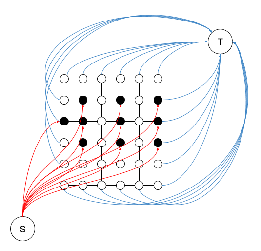
To avoid having to resort to this trick, I changed the problem statement to find m edge-disjoint paths rather than vertex-disjoint. This way, we can immediately modelise this as a maximum flow problem by assigning a capacity of 1 to each edges. In addition, we need to add a source vertex that connects to all of the “starting point” vertices, and a sink vertex that all the “exit vertices” (vertices sitting on the edge of the matrix) connect to.

If we use the first grid above as the input, this is what such a graph would look like:

max-flow

Now that’s a cool graph if I ever saw one!

If we apply a maximum flow algorithm to this graph, we will find a maximum flow of at most m, as there is a flow of at most 1 going through each of the m red edges that start from the source. If we do get a maximum flow of m, then we have a solution for the escape problem, as the various paths going through each of the starting points contain a solution path to escape from that vertex. Those paths are vertex disjoint since there is a capacity of 1 on each edge.

For fun I tried to represent the above problem programmatically. I reused a Python implementation of Ford-Fulkerson that I found on geeksforgeeks. The implementation takes an adjacency matrix representation of the input graph. Our input graph has 38 vertices (6 * 6 + source + sink), so an adjacency matrix would have a dimension of 38 * 38 aka 1444 elements. Now life is too short to hardode a 38 * 38 matrix by hand so I used an adjacency list representation instead and wrote a small function that converts an adjacency list representation of this problem to an adjacency matrix.

#!/usr/bin/env python

import math

class Graph: 
    def FordFulkerson(self, source, sink):
        # <insert FordFulkerson implementation here>

# To convert the adjacency list to an adjacency matrix, each vertex must be 
# assigned an "index"  that will determine their position in the matrix.
# We assign the vertices row by row from 1 to n^2, with 2 additional indices
# for the source and sink.
def get_vertex_index(vertex, adj_list_size):
    grid_element_count = adj_list_size - 2    # minus S and T
    grid_dimension = int(math.sqrt(grid_element_count))
    if vertex == 'S':
        return grid_element_count + 1
    if vertex == 'T':
        return grid_element_count + 2
    # parse 'x,y' string
    i = int(vertex[0]) - 1
    j = int(vertex[2]) - 1
    return i * grid_dimension + j


def adjacency_list_to_adjacency_matrix(adj_list):
    # intialise matrix with 0s
    matrix_dimension = len(adj_list) * len(adj_list)
    adj_matrix = [
        [0 for i in range(matrix_dimension)] for j in range(matrix_dimension)]

    # for each connection, find the index of the 2 neighbours in the matrix 
    # representation and update the matrix
    for vertex in adj_list.keys():
        vertex_index = get_vertex_index(vertex, len(adj_list))
        for neighbour in adj_list[vertex]:
            neighbour_index = get_vertex_index(neighbour, len(adj_list))
            adj_matrix[vertex_index-1][neighbour_index-1] = 1

    return adj_matrix


def main():
    adjacency_list_graph = {
        # Row 1
        '1,1': ['1,2', '2,1', 'T'],
        '1,2': ['1,1', '1,3', '2,2', 'T'],
        '1,3': ['1,2', '1,4', '2,3', 'T'],
        '1,4': ['1,3', '1,5', '2,4', 'T'],
        '1,5': ['1,4', '1,6', '2,6', 'T'],
        '1,6': ['1,5', '2,6', 'T'],
        # Row 2
        '2,1': ['1,1', '2,2', '3,1', 'T'],
        '2,2': ['1,2', '2,1', '2,3', '3,2', 'T'],
        '2,3': ['1,3', '2,2', '2,4', '3,3', 'T'],
        '2,4': ['1,4', '2,3', '2,5', '3,4', 'T'],
        '2,5': ['1,5', '2,4', '2,6', '3,5', 'T'],
        '2,6': ['1,6', '2,5', '3,6', 'T'],
        # Row 3
        '3,1': ['2,1', '3,2', '4,1', 'T'],
        '3,2': ['2,2', '3,1', '3,3', '4,2', 'T'],
        '3,3': ['2,3', '3,2', '3,4', '4,3', 'T'],
        '3,4': ['2,4', '3,3', '3,5', '4,4', 'T'],
        '3,5': ['2,5', '3,4', '3,6', '4,5', 'T'],
        '3,6': ['2,6', '3,5', '4,6', 'T'],
        # Row 4
        '4,1': ['3,1', '4,2', '5,1', 'T'],
        '4,2': ['3,2', '4,1', '4,3', '5,2', 'T'],
        '4,3': ['3,3', '4,2', '4,4', '5,3', 'T'],
        '4,4': ['3,4', '4,3', '4,5', '5,4', 'T'],
        '4,5': ['3,5', '4,4', '4,6', '5,5', 'T'],
        '4,6': ['3,6', '4,5', '5,6', 'T'],
        # Row 5
        '5,1': ['4,1', '5,2', '6,1', 'T'],
        '5,2': ['4,2', '5,1', '5,3', '6,2', 'T'],
        '5,3': ['4,3', '5,2', '5,4', '6,3', 'T'],
        '5,4': ['4,4', '5,3', '5,5', '6,4', 'T'],
        '5,5': ['4,5', '5,4', '5,6', '6,5', 'T'],
        '5,6': ['4,6', '5,5', '6,6', 'T'],
        # Row 6
        '6,1': ['5,1', '6,2', 'T'],
        '6,2': ['5,2', '6,1', '6,3', 'T'],
        '6,3': ['5,3', '6,2', '6,4', 'T'],
        '6,4': ['5,4', '6,3', '6,5', 'T'],
        '6,5': ['5,5', '6,4', '6,6', 'T'],
        '6,6': ['5,6', '6,5', 'T'],
        # Source
        'S': ['2,2', '2,4', '2,6', '3,1', '3,2', '3,4', '3,6', '4,2', '4,4',
              '4,6'],
        'T': []
    }

    adj_matrix = adjacency_list_to_adjacency_matrix(adjacency_list_graph)

    g = Graph(adj_matrix) 

    source = 36    # 6x6 + 1
    sink = 37      # 6x6 + 2

    print ("The maximum possible flow is %d " % g.FordFulkerson(source, sink)) 


if __name__ == "__main__":
    main()

This will print a maximum flow of 10, which is the number of starting points we had in the grid. This means that there is indeed a solution for the escape problem on the input grid. Nice!